A Practical Guide to Two-Sample MR
From GWAS Data to Causal Inference
By Tayyaba Alvi
GWAS Data for MR
Key Data Sources
- GWAS Catalog: A comprehensive repository of published GWAS.
- IEU OpenGWAS: A massive database of harmonized summary statistics, perfect for MR.
Essential GWAS Fields for MR
- SNP Info: SNP ID, Effect Allele (EA), Other Allele (OA)
- Effect Info: Beta, Standard Error (SE), P-value
- Allele Freq: Effect Allele Frequency (EAF)
The Two-Sample MR Workflow
Source: mrcieu.github.io.
Data Harmonization: Ensuring Consistency
This is a critical step to ensure the alleles and their effects are aligned between the exposure and outcome datasets. The harmonise_data() function handles two main issues: strand mismatches and problematic palindromic SNPs.
A. Resolving Strand Mismatches
Correct & Unambiguous
Alleles match perfectly between exposure and outcome datasets.
Exposure
Effect: 0.5
Outcome
Effect: 0.05
Incorrect Reference
Alleles are on the complementary strand. They can be corrected.
Exposure
Effect: 0.5
Outcome (Original)
Effect: -0.05
Outcome (Corrected)
(Alleles flipped to match exposure strand)
Effect: +0.05 (Sign flipped)
Ambiguous Mismatch
Effect alleles match, but other alleles do not. Cannot be resolved.
Exposure
Effect: 0.5
Outcome
Effect: 0.05
B. The Palindromic SNP Problem

Inferrable Palindrome
Allele frequencies are non-ambiguous (e.g., not near 0.5) and suggest a flip.
Exposure
EAF: 0.11
Outcome
EAF: 0.91
Inference: Since 0.11 ≈ 1 - 0.91, the effect allele is likely different. The data is harmonized by flipping the effect sign of the outcome.
Not Inferrable Palindrome
Allele frequencies are ambiguous (near 0.5), so the correct strand is unknown.
Exposure
EAF: 0.50
Outcome
EAF: 0.50
Problem: Impossible to determine if the effect alleles are aligned. The direction of effect is ambiguous.
Instrument Selection: Clumping for Independence
Genetic instruments (SNPs) must be independent. We use a process called LD ClumpingLinkage Disequilibrium (LD) clumping removes SNPs that are highly correlated, ensuring each instrument provides independent information. to select the most significant SNP in a region and remove others in high LD with it. The ld_clump() function handles this.
Manhattan Plot: Visualizing GWAS Hits
Clumping ensures that the selected instruments (green circles) are not correlated due to LD.
Interpreting MR Results & Plots
Scatter Plot
What it shows: The relationship between the SNP effects on the exposure vs. the outcome. The slope of the line is the causal estimate.
Forest Plot
What it shows: The causal effect estimated by each individual SNP. The combined estimate (e.g., IVW) is shown at the bottom.
Leave-One-Out Plot
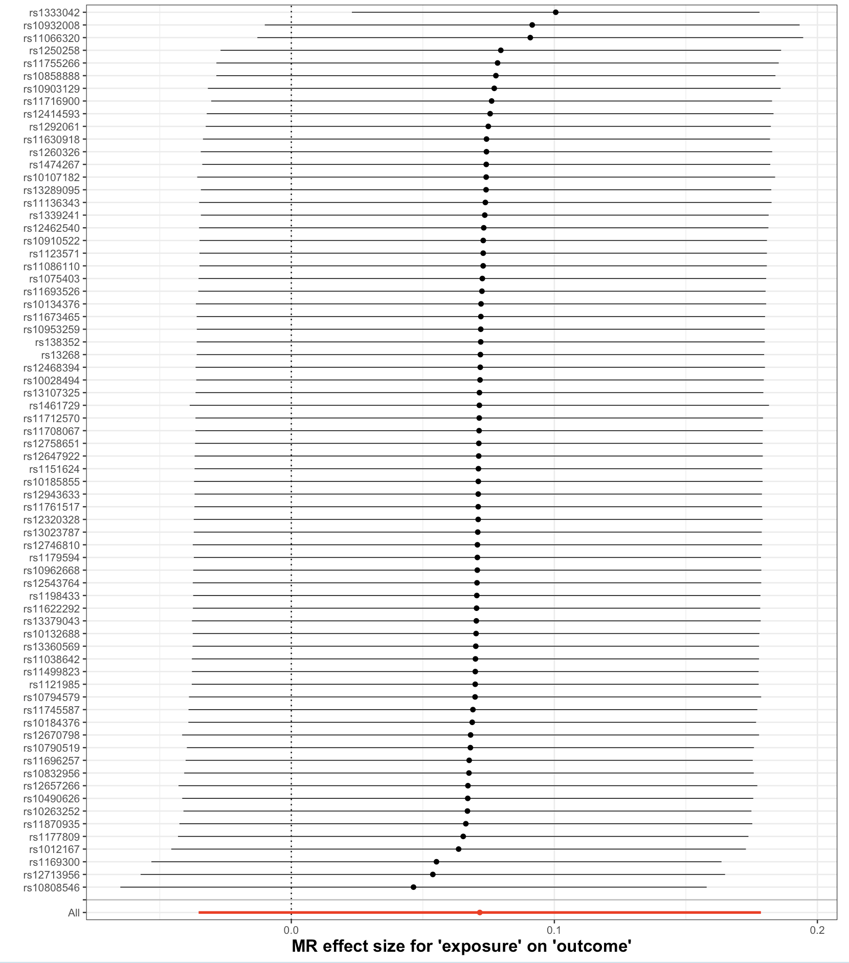
What it shows: Checks if a single SNP is driving the overall result. If all points are consistent, the finding is robust.
Funnel Plot
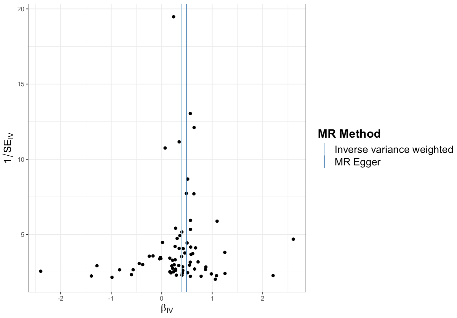
What it shows: Used to visually inspect for heterogeneity and potential directional pleiotropyDirectional pleiotropy occurs when genetic variants affect the outcome through pathways other than the exposure, which can bias MR results.. A symmetrical plot is expected.
Case Study: The IL-6, CRP, & CHD Paradox
The Observational Puzzle
For years, observational studies have shown a strong correlation: higher levels of C-Reactive Protein (CRP), a marker of inflammation, are associated with a higher risk of Coronary Heart Disease (CHD).
↑ CRP → ↑ CHD ?
The Motivation for MR
This raises critical questions that MR is uniquely positioned to answer:
- Is this relationship truly causal?
- Or is CRP just a bystander, confounded by other factors?
- Should we target CRP, or an upstream driver like Interleukin-6 (IL-6)?
IL-6 Signaling & CRP Production

IL-6 is a key upstream driver of CRP production through classic and trans-signaling pathways.
Setting Up Your R Environment
Now, let's test this hypothesis. The TwoSampleMR package is your primary tool. Here are the essential libraries you'll need:
library(ieugwasr)
library(VariantAnnotation)
library(MRInstruments)
library(gwasglue)
library(dplyr)
library(ggplot2)
